This is an attempt to document the steps in a method of imaging for the passive monitor you can make with instructions here, as written in:
Darrin K. Ott, William Cyrs, Thomas M. Peters. Passive measurement of coarse particulate matter, PM10-2.5. Aerosol Science 39 156 – 167 (2008)
Prepping the glass cover slip
Starting from these instructions:
“Sample collection was started by removing the tape tab and ended by re-covering the passive sampler with a clean tape tab. The sample was prepared for analysis in a clean, designated area of the laboratory by removal of the mesh cap and placement of the SEM mount in a holder. The cover glass was marked with a focusing dot just outside of the circle drawn to delineate the boundary of the sample area. This dot facilitated focus of the microscope on the plane of particle deposition. With forceps, the substrate was inverted and placed face down on the center of a clean microscope slide that had been cleaned in the same manner as the substrate described above. The substrate was then held in place on the slide with two pieces of tape. Care was taken to ensure that the tape did not cover the marked circle or the focusing dot.”
Questions arise: How do we draw a circle to designate the boundary of the sample area? What should the slide look like that the slide cover is attached to? I have a fairly definitive answer to the second question, and an inconclusive one to the first question.
Marking a focus point and a circle
marking a focus point is easy. just dab a pen down away from the I tried marking a circle, and it was too hard.

I instead marked four dots at points along the circle while still in the cap. I don’t know how I’d draw a circle after removing from the cap, sitting on a tiny SEM with no adhesive. that just seems beyond difficult. it is very precarious:

I also thought back to the sizing of the Ott et al. sample area vs. the Wagner & Leith sample area. Ott’s sample area is .8mm narrower than Wagner and Leith’s 6.8mm sample area. is that to account for marking under the cap? Ott et al. don’t explain this size difference.
What kind of Slide?
[Ott et al [page 158] suggest taking 40 images over ~70% of the 6mm circular sample on the glass cover slip. What does that look like? I wondered if there was a standard lab procedure. Andrew Maselli suggested a grid on a slide. I looked up standard grid slides and grids of the size “one low-powered field” (100X) are 1.45mm wide.

Laying such a grid across a 6mm circle, the size of our sample area, it appears that there are 40 complete squares, and that the circle is roughly 55 squares in area, so the fields represent ~70% of the sample area.

It seems the glass cover slip should be taped face down on a low-powered field grid slide. but…
Can we capture a full low powered field grid in one image?
Ott et al. (pg 158) imaged the slide at 1064 x 1280 pixels at 100x optical resolution (10x objective lens), with a resolution of 0.524μm per pixel. This is a 557.5μm x 670.7μm stage, about 1/5 the size of a 1450μm “low power field” sample size…
I don’t really know what to make of that.
Imaging the slide
Andrew Maselli suggested focusing down the the plane of the grid, centring a grid square, then focusing up to the plane of dust and imaging there. This requires setting a focus height for the focusing dot, and returning to that height.
The light of the microscope will also have to be focused on the dust plane.
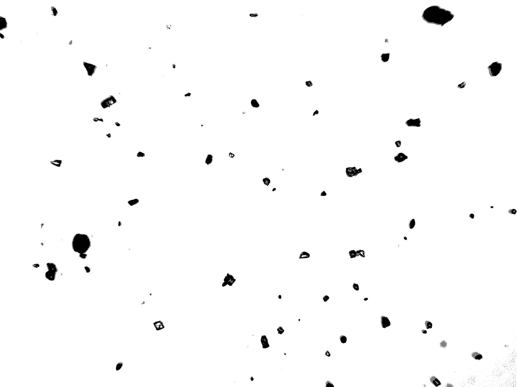
Andrew Maselli also suggested using the “bright field” setting on the microscope, which produces a nice high-contrast image. This image taken with a Zeiss Axial Observer z1, a very expensive microscope.

compared to a color image taken with a less expensive Zeiss Axioskop which costs about $1000 used:

Both of these would probably work well with the software, where we’re going to be sizing particles in ImageJ, and will need some custom algorithm that makes a strong threshold between light and dark and ”fills holes,” or light spots in otherwise black particles on a white background.
The light field image produces clearer particles:


Next steps…
Using ImageJ and extrapolating mass concentrations!
Ott et al validated their process by imaging NIST traceable 5-μm borosilicate glass microspheres (Catalog # 9005, Duke Scientific, Fremont, CA).
3 Comments
One possibility in order to get a clearer image is to try using the "threshold" filter in photoshop, or photoshop elements, GIMP, etc. It's helped me trace dust plumes in photos of sand mines, although that's a completely different scale. Too bad I could never offer proof that silica particles brightened and diffused sunlight.
Reply to this comment...
Log in to comment
I'm writing up an introduction to particles in the air right now (rough draft), and one of the questions I wanted to answer was about naked eye observations of particles.
There should be a diffusion effect when particles are between the range of 1-10μm. There must be some regular ways of qualitatively assessing small particles through measuring some aspect of their diffusion.
This EPA document on atmospheric visibility talks a bit about light extinction, and briefly describes assessing visibility by taking pictures of targets 1-10km away through telescopes.
http://www3.epa.gov/visibility/pdfs/introvis.pdf
its a compelling idea to document haze as a pollution proxy. I want to learn more!
Reply to this comment...
Log in to comment
You don't state what happens with the 40 images taken. Are they stacked together for analysis or they are analysed individually.
Reply to this comment...
Log in to comment
Login to comment.