Using a webcam or a pi camera, it quickly becomes clear that a single capture cannot encompass the large range of brightness in the scene, also known as the dynamic range. A solution is high dynamic range (HDR) imaging, a process that combines data from multiple exposures into one image that is neither overexposed, nor underexposed.
Previous notes that have discussed HDR include: HDR: In search of high-er dynamic range by stoft and High Dynamic Range (HDR) Imaging (revisited) by MaggPi.
This post extends the method described by MaggPi using the same OpenCV library for python, and focuses only on the Debevec algorithm. Debevec and Malik (1997) wrote an excellent paper on their algorithm that is very helpful to understand the method: Recovering High Dynamic Range Radiance Maps from Photographs
The Debevec Method
In brief, the algorithm is based on the principle that camera sensors have a non-linear response to light. That means, if you double the light energy in the environment, the pixel value is not doubled. For research where we are trying to extract information about the world using pixel data, it is super important to know how pixel values map to irradiance in the captured scene.
Debevec and Malik's method produces a function, and when plotted on a graph, the x axis represents pixel values (from 0-255) and the y axis represents sensor exposure, which is a product of scene illuminance (E) and shutter speed (Δt).
The steps include:
- Taking a series of photographs with known and different exposures of a scene with the same camera position
- Collect a sampling of pixels from the scene, and determine each pixel's value for every exposure time. This works even though we don't know the actual irradiance value for any pixel, since we assume that the scene irradiance is constant across the photograph set.
- Use an algorithm to combine the pixel data into a beautiful curve.
While steps 1 and 2 are straightforward, I found the algorithm quite complex which turns the graph below from the left to the one on the right. It's so great that it's already implemented in OpenCV! I mostly followed the code from this tutorial: https://www.learnopencv.com/high-dynamic-range-hdr-imaging-using-opencv-cpp-python/

Figure from Debevec and Malik 1997
This curve can then be used for any image set to map pixel values back into irradiance (E) since we know the sensor response function (f), the pixel value, and the shutter time (Δt) where
pixel value = f(E * Δt)
So what's the catch? In order to produce this sensor response curve, we need a suitable set of images, ideally over a wide range of exposures that overall contain data for each color (r,g,b) ranging from 0 - 255 values. We probably don't want to do this kind of elaborate process all the time, and that's why we can separate it into two steps. First, generate the sensor response curve. Then, save the response curve, and use it in the future to process all of your HDR photos.
The importance of a good photo sample is demonstrated in the 3 images below, ranging from poor to very good:

The cropped CFL image is better than its uncropped counterpart because the random sampling is more likely to fall on pixels with a greater variety of information. The LED image is much better than the CFL data because it has a broader spectrum, and using a wider exposure range, there is much more data for each color ranging from 0 to 255.
Just for comparison, here's also a Canon sensor response curve generated from a set of HDR photos found online:

Source images copyright by Wojciech Toman: http://hdr-photographer.com/hdr-photos-to-play-with/
I don't know if the PublicLab webcam is capable of manual control, but if it is it would be interesting to see its response curve too.
Generating an HDR image using the sensor response curve
Now that we have the sensor response curve, we can take any image and map it back into irradiance values. While they won't be representative of absolute irradiance (e.g. energy units) without further calibration, they will be proportionate to each other.
You only need two lines of code from here:
mergeDebevec = cv2.createMergeDebevec()
hdrDebevec = mergeDebevec.process(images, times, responseDebevec)
where images is your image set, times is their exposure times, and responseDebevec is the .npy array from the response curve we generated earlier. The output, hdrDebevec is now a numpy array containing the merged HDR data.
From here we have two choices:
A) Compress the data into an LDR (i.e. remap the values to 0-255) to present as a .png image
B) Directly extract the data from the HDR numpy array
Option A is nice because it's easy and you can see the pretty picture, but Option B will have better data resolution since we are not compressing the irradiance values. Let's compare them. For each, I've extracted data from the same pixel row.
Creating the LDR and saving the image is only 3 more lines of code using the OpenCV library as cv2:
tonemap = cv2.createTonemap()
ldr = tonemap.process(hdrDebevec)

cv2.imwrite('hdrHolo1.png',ldr * 255)
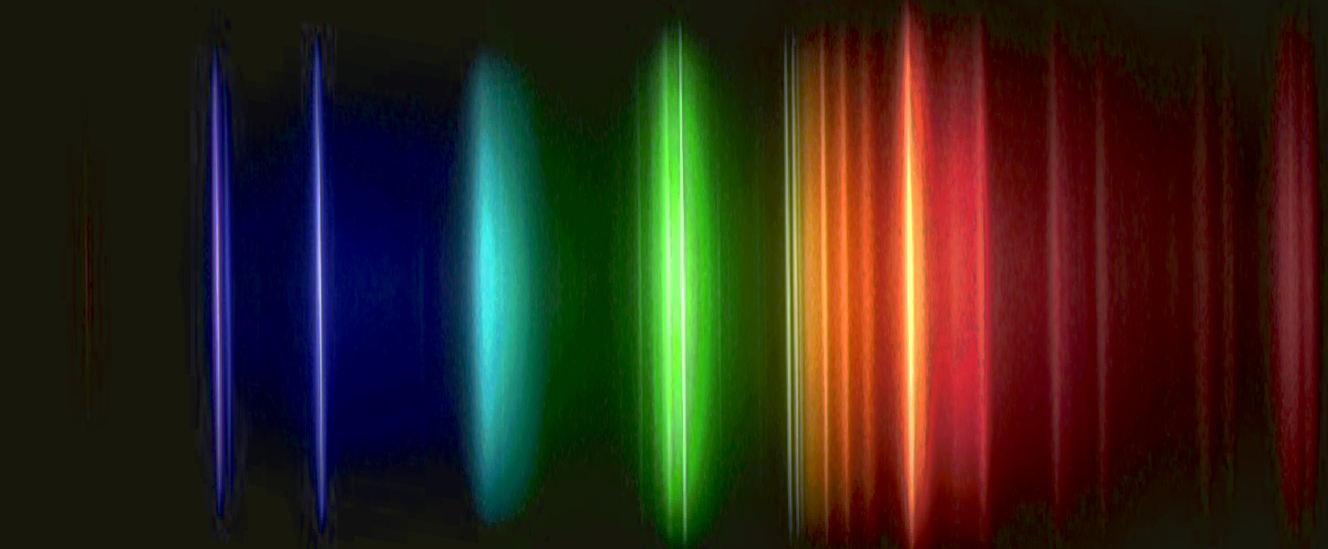
The uploaded spectrum is available on Spectral Workbench, where I extracted one line of data. https://spectralworkbench.org/spectrums/160042

The peaks are sharp and the shape is good, but the final test is the data comparison.
The HDR Plot

exported from python
The LDR Plot

extracted from the png uploaded to spectral workbench and plotted in Excel
Wow, for two things. Firstly, the HDR plot looks great. Secondly, a lot of data was lost in the compression stage. After all that work, it's really not worth it to discard all that great data.
So in conclusion, this process is promising, but the best data relies on a) manual control of your camera b) a good dataset for sensor calibration and c) using the HDR data directly without compression.
In further study, I am interested to know if getting the raw RGB data from the pi before jpg compression will be even better, since I am suspecting that certain dips next to the tallest peaks are due to compression.
Appendix:
I attached a screenshot of my camera settings on the pi camera web interface: IP_Camera_Settings_Pi_annotated.pdf
14 Comments
@warren awards a barnstar to jenjimah for their awesome contribution!
Reply to this comment...
Log in to comment
Good work and observations. Yes, I think HDR techniques can help extract additional dynamic range from these simple cameras. In reading through your notes I'm also wondering about some fundamentals which I'd noticed in my own experiments. Web-Cams are designed and optimized for taking images of 'world scenes' not spectra from diffraction gratings and so they tend not to react 'nicely' to such input. I suspect the Pi camera is much like other 'web cams' since they are all based on similar sensor chip technology.
The cameras have internal AGC loops (Automatic Gain Control) which seek to 'level' the analog gain in ALL pixel elements based on an overall image intensity average. This makes the camera output both a function of the specific 'scene' and a function of an active loop with an unknown, and even variable, loop bandwidth (rate of correction).
With one camera I used + a matlab interface, I was able to shut off the AGC and set a fixed image gain. At that point, the camera's response was quite linear (for such a simple detector) ..... but with AGC running, the camera did appear to be non-linear -- and difficult to control. (This can appear as instability in the spectral intensity over time -- which most tend to just average out, but which really shows as a significant intensity error value to the final data.)
The other factor, once the gain is fixed, is handling 1) the gain step size (another calibration) and 2) noise which tends to increase as the gain increases (a limit to the range of an effective HDR).
So, I'm just suggesting that it would be good to know if the observed non-linearity is a result of an active AGC loop. If it is, then the 'correction' could be further complicated by not having control over the specific range of the AGC's operation -- which is, in turn, a function of the image detail being observed (a variety of spectra with variable average intensities). True, extracting accurate data is not terribly straight-forward ;-)
Great question, it's pretty amazing you were able to shut off the AGC circuit. I had previously imagined that most ofthe pre-data export operations were hardwired or hardcoded in.
Yes it looks like the Debevec algorithm just jumps right over top of the camera functions and wraps it all into one to get from scene illuminance to sensor data. They acknowledge this in their paper.
"Digital cameras, which use charge coupled device (CCD) arrays to image the scene, are prone to the same difficulties [as film]. Although the charge collected by a CCD element is proportional to its irradiance, most digital cameras apply a nonlinear mapping to the CCD outputs before they are written to the storage medium. This nonlinear map- ping is used in various ways to mimic the response characteristics of film, anticipate nonlinear responses in the display device, and often to convert 12-bit output from the CCD’s analog-to-digital convert- ers to 8-bit values commonly used to store images. As with film, the most significant nonlinearity in the response curve is at its sat- uration point, where any pixel with a radiance above a certain level is mapped to the same maximum image value."
But the question still remains about how stable is the sensor response curve for our cameras? I guess we can really only know for sure through testing. Test the camera in a variety of situations and compare. Even better would be to test multiple cameras to see the quality control, to test if it could make sense to use one sensor curve and apply it to other people's hardware. That would really reduce the workload required to start doing hdr, although my hunch is it's probably still better to have a customized curve for each individual sensor.
Is this a question? Click here to post it to the Questions page.
Right, the camera's do automate as much as possible, which works against the needs of spectrometers. If the AGC cannot be shut off, then it becomes very difficult to make intensity measurements (even relative intensity) because the chip is intrinsically modifying the gain without knowing when or by how much.
In a simplistic way, it is easy to see the spectral curve change level with a change in source light -- even with an AGC. That is usually because the adjustment range of the AGC is limited to less than the sensor's dynamic range. However, when looking for small intensity changes, the data will be a mix of effects of both the AGC (which is typically based on average 'scene' intensity) and real changes in input light intensity. They are co-mingled and not easily separated.
I believe that an intensity correction curve is only possible if the gain can be controlled. I was not sure by the above description if the python code had some interface for the PI camera for switching the AGC off and for controlling the gain. Might look for that and/or do a bit of web search on controlling those parameters in the PI camera. Sometimes camera chips have the option but the chip interface card does not allow them to be programmed. Some cameras do.
Hi, just in case you didn't see this I recently came across this, which could be helpful maybe?
https://gitlab.com/bath_open_instrumentation_group/picamera_cra_compensation
Is this a question? Click here to post it to the Questions page.
Thanks! I just had a look at their manuscript. There are a lot of details there that I had no idea about and need to learn.
@stoft I tried reading about the raw RGB ouput on the picamera documentation but I did not find the description to have too much information, but maybe I just need to read more. To me it seems like a black box right now and hopefully by reading we can gain more confidence about how to control the camera consistently. That link @warren posted seems like it has quite bit of good info that is not found on the pi documentation.
From that link, I found a 'settings' file here:
https://gitlab.com/bath_open_instrumentation_group/picamera_cra_compensation/blob/fdb98308149e686ac539db8e411bf2d2eafa9b0c/data/monitor_and_50mm_lens/neopixel_jig/camera_settings.yaml
which appears to set the camera: analog gain, white-balance, digital gain, exposure off, some 'state' settings, etc.
However, a quick web search found the picamera docs:
https://picamera.readthedocs.io/en/release-1.13/fov.html
which describe setting the exposure to off to stop the auto-gain adjust ... so there do appear to be some useful controls.
Just a thought: Using other's code 'packages' can have the pitfall of not having process control that is well understood. So, one suggestion is to write some new basic camera control code, in python if you like, which 1) does the camera setup, 2) controls the cam to get images, 3) extracts a set of 'pixel lines' through a spectra and 4) manipulates that data to construct the three R/G/B spectral raw data arrays. That is the root information you can and need to control. Most all remaining code is thus just requesting spectra (via your root code) and manipulating the resulting extracted raw RGB data. Some 'package' from the web is thus just a utility to try out (though you might have to isolate their core feature you want so as to integrate it onto your code). This helps isolate the functionalities, validate the basic camera-spectra building blocks and to know precisely how the data was obtained, its accuracy and its error limits. Just a thought ...
Ah yes! For a moment there I was confused between what the paper was saying about non linearness applied to pixels prior to data export and AGC. I see they are two very different things. Yes the photos in this post would have been impossible to take if AGC was on. Using the cam software that comes with pi builder, you can turn off the exposure mode which turns off the AGC, so you can set exposure time, resolution, and iso manually. I should post a screenshot of my settings at the bottom there in case anyone wants to see or copy. I had everything controlled except for shutter speed, just like a regular manual camera. But I agree about having a dedicated software that is even more raw because the ip control face does not allow for long exposures for some odd reason, nor raw data export, and its a bit unclear about which settings override other settings (though you can read it in the docs) so that's why I am leaning towards a different/custom data extraction program too.
In the code of the pi camera library, which is what many of the other libraries are built on, there is a special data export option called .array which allows for raw rgb data export as a numpy array. You can export this and a list of the metadata which is basically all the info you need for data processing. One limitation is it says you cannot export full frame photos in rgb as it results in an out of memory error since the files are so large, so you have to crop it or choose the extraction line first. You can however export full frame photos in the alternative YUV raw format, but that requires further processing on the PC end to turn it into RGB. I thought maybe cropping first and then having the pi send it over in smaller files would lead to a faster process.
Here is the link to the picamera.array module https://picamera.readthedocs.io/en/release-1.10/api_array.html
Oh, i'd love to see this, thanks!
Done!
Yes, once the camera exposure is under control (and fixed value) then the linearity can be measured -- IF you have controlled means of adjusting the input light level (eg. say a neutral density filter of known attenuation, then use N=1,2,3,4... filters). Mapping of gain settings to output level could be done after that.
On capturing image data: Yes, extracting entire images is a waste of bandwidth. I'd suggest doing 2 steps: 1) extract a 'band' of image lines (eg. 16) that are 'centered' in on the spectrum, then 2) operate on that line data to extract a single spectrum.
The second step is important because just any single pixel line will include camera noise, optical errors from having discrete lines of pixels and the uncertainties of the mechanical stability of the spectrometer. I found that the 'peak' data response for a spectra generally never aligned with any single line of pixels. (Recall that the pixel sensor areas are small physical areas, separated from each other, so it is an array of 'spot-points'; not contiguous detection areas. So, the step #2 gives room for an algorithm to process a set of parallel pixel lines in an adaptive way prior to any other processing (which will be assuming the spectrum is accurate). I published notes on a number of related techniques which might give some helpful ideas.
Reply to this comment...
Log in to comment
Hello, I thought I'd chime in after your shout-out of the work we're doing. Our OpenFlexure eV software does attempt to get as close as we can to manual control over the Raspberry Pi camera. A few things that might help clear up some confusion:
the picamera library does not yet support changing the analogue gain or lens shading correction. However, I have a fork (and a merge request) that adds these features. There are good reasons it's not been merged yet - but if you want to use them you can find them here: https://github.com/rwb27/picamera/releases/tag/v1.13.1b0
the picamera.array submodule is great, but beware that anything except PiBayerArray is not actually raw data. That is made clear in the docs, but it's easy to forget about.
I really should tidy up what we've done into some neat, easy-to-extract scripts along with the manuscript, and I hope this will be done soon. I am working on the manuscript today, and it is finally getting there!
Reply to this comment...
Log in to comment
Login to comment.