Detection of Metals in Water using WheeStat
Purpose:
The purpose of this wiki is to describe a good, general method for determining the concentration of metal ions (copper, lead, arsenic, etc ) in water that is amenable to use by the DIY / environmental activist community. Electrochemistry has a long history of use for this type of application and the WheeStat and other low cost potentiostats have been developed that can be built or bought for reasonable amounts of money.
Some links describing the WheeStat are available on the PublicLab site. The online user's manual is here. Kit assembly instructions are found here. Directions for setting up the WheeStat are here.
Overview:
While a number of electrochemical methods can be used to determine the identities and concentrations of metal ions in water, one of the best is anodic stripping voltammetry (ASV) with the Standard Additions Method.
The voltage profile for the ASV experiment is presented in the figure below. In this figure, time is on the x axis and voltage is on the y axis. Before the experiment is started, the working electrode should be at "open-circuit voltage". That is where no current flows (not necessarily zero versus the reference electrode). In this figure, open circuit is represented to be -100 mV. The experiment is started at time zero, when the applied voltage is stepped to +400 mV to strip the electrode of all reduced material. This is important when using the mercury film electrode as described below in Example Method 2. After 2 seconds at +400 mV, the potential is stepped to the starting voltage (-800 mV in the figure) where it is held for the "initial delay" time specified in the user interface. For the figure below, that is 8 seconds. During the initial delay, the material to be analyzed is deposited onto the electrode for later analysis. At the end of the initial delay there is an additional 0.5 seconds of "quiet time" before analysis begins. During the analysis stage, the voltage is ramped from its initial value (-800 mV) to its final value (0 mV), during which time, current data is collected and displayed. After the analysis stage, the applied voltage is returned to the open-circuit value. While the analysis stage in this figure is represented as a continuous ramp, the WheeStat uses a differential pulse profile to acquire data.

To use the WheeStat you will collect a water sample of an unknown metal concentration and run an anodic stripping voltammetry experiment on this sample to generate a voltamagram. Then you will spike the sample with a known concentrations of the metal of interest and generate a voltamagram for each spiked sample. From the peak areas of the generated voltamagrams the concentration of the metal of interest in the original sample can be determined.
Things you will need:
• WheeStat and a computer running the WheeStat software
• Electrodes (working, counter, and reference)
• Supporting electrolyte (something like potassium chloride, KCl)
• Metal of interest (something like copper nitrate)
• Something to accurately measure volume (graduated cylinder, syringe, pipet…)
• Beakers or bottles to make solutions in
• Deionized or distilled water
• Sample to analyze
Method Example 1
Determining the concentration of copper in stream water:
The first thing to do is collect a water sample to be analyzed. To do this you want to take a clean container, rinse it three to four times with water from the river/lake/pond/etc. that you will be analyzing. After rinsing the container, you can then fill the container with whatever water sample you want to analyze. Be sure to record when and where you took your sample.

The second step is to make some stock solutions that will be added to the water sample (for information of how to make a solution go here). The first stock solution is one of just a supporting electrolyte in deionized or distilled water. In the example data a 0.2 molar solution of potassium nitrate in deionized water was used.

The second solution is a known concentration of the metal to be analyzed (copper nitrate in the example data) in some of the supporting electrolyte solution mentioned above. This sample will be used to spike the unknown water sample. The concentration of the metal in this stock solution will need to be determined experimentally, and will depend on the concentration of the metal in the unknown water sample and the type of type of equipment you have available to measure accurate volumes. In the example data, an 8.2 mM solution of copper nitrate was used.

The next step is to make a series of samples to be analyzed with the ASV method. Each of the samples should have the same volume of unknown sample, same total volume, but with varying amount of electrolyte and metal-electrolyte solution. A table of the volumes of used of each solution for the example data is shown below.

After the solutions are made, connect the alligator clips of the WheeStat to the appropriate electrode (black-working, green-reference, and red-counter). In the exaple data a silver wire with heat shrink was used as the working electorde, a graphite rod was used as a counter electrode, and a silver/silver chloride reference electrode was used.

Next insert the electrodes into the solution with just the unknown water sample and supporting electrolyte.

Start the WheeStat software, select the COM port corresponding to the LaunchPad, click the "Connect" button.

Select the ASV experiment from the dropdown list.

Adjust the parameters (will need to be adjusted experimentally), and start the run.

After the voltamagram is finished, save the data, and repeat the steps for solutions two through four (or however many solutions you may have).


There should be a peak in the first voltammagram that grows in intensity as the concentration of added meatal increases.

The next step, after you have generated a voltammagam for each solution, is to find the areas of the peaks in the voltammagrams which correspond to the metal of interest. A GUI to do the integration will be available soon, but for now, integration can be done in excel. If there are no overlapping peaks with the peak for the metal of interest, then the trapezoid integration method can be used. If there are overlapping peaks the data can be fit to and equation using the Solver function in Excel (using equations 1 and 2 in this link).
Next is to graph the concentration of standard metal solution added versus the peak areas. This plot should be linear and look something like the example data below.

Once the data is plotted. Fit the graph with a linear line. From the slope and intercept of this line the X-intercept can be found. The absolute value of the X-intercept is the concentration of the metal of interest in the unknown sample.
In the example data above the X-intercept occurs at -0.27, since the x-axis is in mM, the concentration of copper in the sample with only the unknown water and electrolyte is 0.27 mM. Since the unknown water sample was diluted by a factor of two with the electrolyte solution, the actual concentration of copper in the unknown water sample is 0.54 mM.
Method Example 2
Measuring lead in water.
Improvements in the sensitivity of the experiment are possible. Electrode materials and solution conditions will affect your ability to measure low metal ion concentrations. Conditions have been worked out to co-deposit your metal of interest with mercury in low concentration of dilute nitric acid. The procedure for this experiment was taken from this web site. Notice that we used a commercially available glassy carbon electrode in this experiment The graphite sticks that we have used under milder conditions appear to react under the conditions and are not suitable for use in nitric acid. Glassy carbon electrodes can be purchased from CH Instruments for ~$88 with shipping. For this experiment, we will need a stock solution containing 0.1 M KNO3, 0.05 M HNO3 and 40 ppm Hg(NO3)2 in deionized water. If you do the math, you will find that you will need to weigh out a very small amount of the mercury salt to get a liter of solution at this concentration.. The easiest way to make the stock solution is to dilute a more concentrated solution. I made the more concentrated solution by dissolving 0.29 g Hg(NO3)2 and 0.16 mL HNO3 in 50 mL de-ionized water. This gives a solution that is 3400 ppm in Hg. To make the stock solution, I added 15 mL of this solution, 10.7 g KNO3 and 3 mL HNO3 to about 500 mL water, stirred it up, and diluted to 1 liter. This stock solution was used to make up all the subsequent solutions. A series of lead containing solutions were prepared by a method called serial dilution. First, I weighed out 0.28 g Pb(NO3)2 into a 25 mL volumetric flask, dissolved it in stock solution and diluted to the mark. This was Pb solution 1. Pb solution 2 was made by diluting 1 mL of the first Pb solution to 10 mL with stock solution. Pb solution 3 was made by diluting 1 mL of Pb solution 2 to 10 mL. This gives a solution that is 2.8 ppm in Pb. Test solutions were prepared by 1:2, 1:4, 1:8, 1:16, 1:32, and 1:64 dilutions of Pb solution 3. Annodic stripping voltammagrams were recorded for each test solution using the following conditions; initial voltage; -800 mV, final voltage; 0 mV; preconcentration time; 30 s, scan rate 400 mV/s. The figure below shows a screenshot of several overlayed voltammagrams from a solution containing no Pb and from solutions with Pb concentrations ranging from 44 to 700 ppb.

While repeated measurements were made for each sample (as seen in the screenshot), only one voltammagram per sample was saved for analysis (as a .csv file).
Data Analysis:
I really should be using the program that Ben wrote to analyze this data, but when you get to be my age, It is hard to let go of the old ways.
Anyway, here is the brute force method: When you open the csv file (using excel) you should see five columns of data. If all the data is all in one column separated by commas, select that column, go to the data tab and find the "text to columns" icon. Clicking on that icon will open a dialog box that will allow you to convert the data to columns. Make sure you specify that your file is delimited by commas.
You should now have five columns. They are voltage, high current, low current, max current and min current. While the GUI displays a single line for each voltammagram, two y values are recorded for each x value and the displayed y data is the difference between the two recorded y values.To illustrate data analysis, consider the data in the following figure. On the right is a plot showing the two sets of raw data. In the center is the plot of the difference between the two current readings. Notice that there is a solid line representing a baseline under the data points. The right hand plot shows the peak after the solid line is subtracted from the data. This baseline corrected data is then modeled using the equation below:
i(calc) = A{exp(s(E-Eo))/(1+exp(s(E-Eo))2

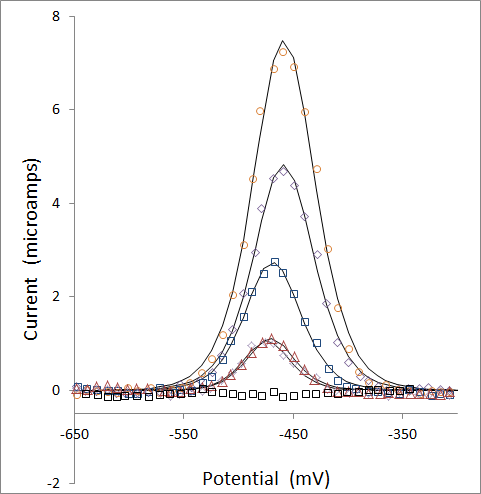
Baseline corrected data and the best fit curves are presented below for the voltammagrams of Pb solutions at zero, 44, 88, 175, 350, and 700 ppb. Note that the 44 and 88 ppb data overlap strongly, giving the impression that there are fewer points than are there.

Once the data has been modeled, peak areas are calculated from the best fit parameters of A and s from the equation above: peak area = A / s
The plot of peak area versus Pb concentration for this experiment is presented below:

While the correlation is not perfect and does not extend to the 15 ppb drinking water action limit established by the epa, further refinements of the experiment are possible. Further, I think the data look pretty good, especially given the the instrument and electrodes cost less than $200 combined.