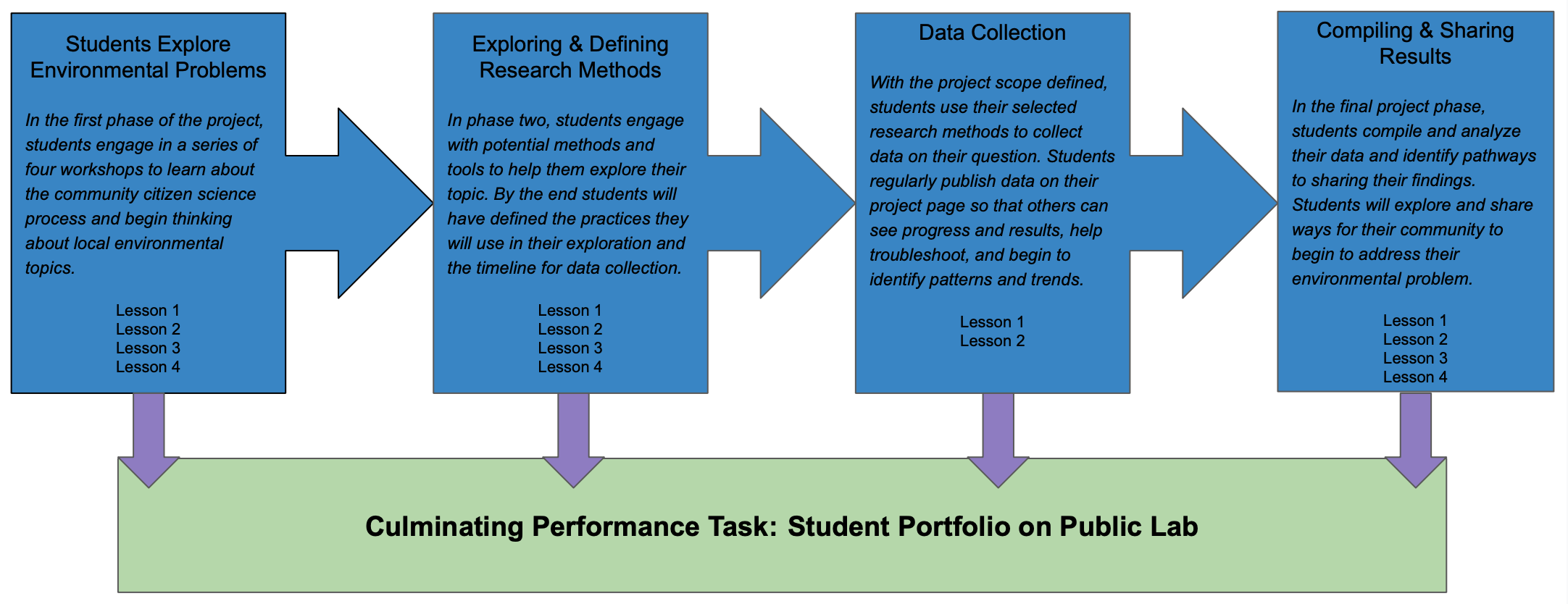
This lesson is part of a series of lessons designed for educators to facilitate student-led inquiry around environmental topics. If there are time constraints, this lesson can be split into two at the Elaborate portion of the lesson. During Phase I of this series, students work towards identifying and learning about environmental topics.
You can learn more about this series here.
You can access this lesson plan as a Google Doc here.
Overview
Time: 105-125 minutes
Materials:
Computer/tablet with internet access (ability to share screen with class is a bonus).
Access to Google Trends and CODAP (start-up guide here).
Guiding Question: What story does our data tell?
Objective: Complete data analysis and identify trends in the data. Students will also begin planning on how to share the data with their community and online networks.
Engage
Time: 10 minutes
Exploring Trends
Ask students what the last thing they googled was. Pick an example to search on Google Trends. use the question mark next to "interest over time" to dicuss what is being displayed on the chart. with the students, explore both display modes: over time and by region. You can hover over a point on the map or place on the map to see data for that selection. Ask for a second display term and how this comparison of information changes the charts.
Explore
Time: 10 minutes
Interpreting Trends
Make sure that all students can see the graphs of your search term trend. Have students each write a one sentence summary of what this data tells them. Ask a selection of students to share what they've written and identify what about the graphs communicate that piece of information.
Explain
Time: 25-30 minutes.
Working with Our Data:
Have students pull up data from their shared data storage site. Because this sheet shows raw data entered online by their fellow students, there may be some mistakes and inappropriate data values in the data sets. Before analyzing your data and making conclusions, make sure to take time to oversee and clean your data. You'll want to correct spelling mistakes and handle any missing values. Create a Plotbox for each variable of interest to visualize the distribution of your data and any outliers. You can use this worksheet to create a Box Plot and identify potential outliers using the free online software, CODAP.
Graphing the Data
Using CODAP, we can create and save graphs very simply. we can create these graphs on teh same sheet as our Box Plot. On a new graph (created by pressing the "Graph" button on the top toolbar) we can create a new graphing space. You can drag variables (called "Assets" in CODAP) onto the different axes to graph them. You can graph more than one variable on the X axis by dragging the second variable onto the second axis. CODAP can create a variety of graphs which are accessible via the paintbrush menu on the graph toolbar.
If you'd like to make your graphs in Google Sheets, here is a walkthrough for creating a graph and information about the different types of charts and graphs available. If you prefer Microsoft Excel, this website has information on creating Excel graphs.
Elaborate
Time: 30-45 minutes
Exploring Our Data:
Data Analysis
Exploratory data analysis helps to understand the data better. You can use this chart to begin your data analysis journey. The above link also has resources for more in-depth data analysis.
Discovering Trends
The purpose of collecting data is often so that we can identify patterns, like numbers trending upwards or correlations between two sets, in order to draw conclusions about the data set. Sometimes a trend is easy to spot within a table. When that's not the case, visualizing the data in the form of a chart can help us to more clearly see a trend.
Tips for Identifying Trends in Tables
Sometimes a table can be an effective way to visualize trends in your data. Organizing your data can help make these trends more clear. In programs like Google Sheets and Microsoft Excel, you can sort the columns of data by date or value to help tease out trends.
Conditional formatting can also be a powerful tool for trend visualization. With conditional formatting, cells, rows, or columns can be formatted to change color if they meet certain conditions. For example, you can have a row turn green if a value is below a set threshold, or set a color scale based on a minimum and maximum value. To learn more about applying conditional formatting in Google Sheets, see here, or for Microsoft Excel, see here.
Identifying Trends in Charts
Upwards and downwards trends in charts can be easy to identify when the relationship is largely linear. The graph below, from Gapminder, showing fertility rates in India. This a clear example of a downward slope.
Other charts might show a large amount of fluctuation over time. It can help to add a trendline to view the major changes. You can quickly add trendlines in Google Sheets as well as in Microsoft Excel.
Evaluate
Time: 30 minutes
Improving our Models
Now we will go back to our logic flow charts from the beginning of this series and expand them based on what we learned. To do this, we will create updated models in Sage Modeller. This will allow us to build dynamic relationships and import our data into the model. This interface is very similar to that of CODAP. To learn more about Sage Modeller, check out the How-To Guide or the Getting Started Video. An expansion of the lesson two example can be found here: Example Model.
0 Comments
Login to comment.