Analysis Prep
In analyzing passive particle monitors, we’ll collect a glass slide cover with a 6mm circle of dust that has settled over 1-10 days in a passive particle monitor we've imaged.

We’ll take a survey of 40 images (see note on imaging) of the glass slide cover at 100x:

We’ll then process the images in full-contrast black and white and fill any “holes” in the image so that the image can be processed more easily. We’ll use ImageJ, which may have standard functions for contrast if not hole filling, though Ott and Peters used it to do that.

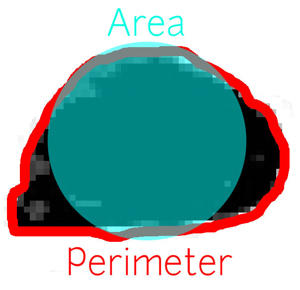
Each individual particle will be sized as if it was a circle of the same area (projected area diameter) as the as the particle's outline (the projected area) and measured for circularity. Circularity is a ratio of the area to perimeter: 1 / (4π gravity x Area / Perimeter2) Again, we’ll use ImageJ, which should have standard functions for this.

At this stage we’ll know:
- number of images x image area = survey area
- number of PM2.5 & of PM10 -sized particles on the survey area
- time the monitor was exposed.
we want to figure out what the average mass concentration of dust was in the air over the sample period, in a micrograms per cubic meter (μg/m3) equivalent.
We’ll be following the mass concentration analysis used in on field samples in Ott et al. I’ve tried to collect a procedure, for a deeper explanation please read the paper:
Darrin K. Ott, Naresh Kumar, Thomas M. Peters. Passive sampling to capture spatial variability in PM10–2.5. Atmospheric Environment 42 746–756 (2008)
…with supplementary information from its references:
Darrin K. Ott, William Cyrs, Thomas M. Peters. Passive measurement of coarse particulate matter, PM10-2.5. Aerosol Science 39 156 – 167 (2008)
Jeff Wagner and David Leith. Passive Aerosol Sampler. Part I: Principle of Operation. Aerosol Science and Technology 34: 186– 192 (2001)
Jeff Wagner and David Leith. Passive Aerosol Sampler. Part II: Wind Tunnel Experiments. Aerosol Science and Technology 34: 193– 201 (2001)
I’ve used annotation that is more “pseudocode” than math annotations in text, and then drawn the symbolic math by hand because I don't know how to do math annotation on a computer (this research note probably accepts LaTeX syntax but i don't know it)
Calculating Individual Particle Mass
the mass of the particle is a volume times particle density, corrected for the relative circularity of the particle:
Mass = (π/6) x particleDensity x (projectedDiameter / ParticleCircularity)3

particle circularity is: 1 / (4π gravity x Area / Perimeter2)
We know the projected-area diameter and circularity of each particle, and we can assume, as Ott et al. and Wagner & Macher 2003 did, that dust is 2g/m^-3.
They assume this number because particle density has a smaller effect on the results than other factors and is hard to know over a varied sample period. We can pick a different concentration from the literature or based on test results of background dust characteristics from a filter-based assessment (more on page 157, Ott et al.).
Calculating a particle’s contribution to the mass concentration
The Contribution of the particle is the mass flux of the particle divided by its deposition value
Contribution = massFlux / depositionValue

unpacking this (explained below) into one equation, we get
Contribution = [Mass / (sampleArea x Time)] / [ [[(particleDensity x projectedDiameter2) / (18 x dynamicViscosity)] x g] x .00595 x [[projectedDiameter x [(particleDensity x projectedDiameter2) / (18 x dynamicViscosity)]g] / kinematicViscosity]^-0.439 ]

I could use help understanding what the kinematicViscosity or dynamicViscosity are, all other numbers accounted for
Mass Flux of the Particle
I don’t really know what mass flux means but its the mass of a particle divided by the total sample area times the total sample time:
massFlux = Mass / sampleArea x Time

Deposition Value of a Particle
The deposition value of particle is the ambient deposition value multiplied by an empirical “mesh factor” derived in a wind tunnel data in Wagner and Leith Pt. II.
depositionValue = depositionAmbient x meshFactor

Ambient Deposition factor
Ott et al. ’s deposition factor is the “relaxation time of the particle” multiplied by gravitational constant.
depositionAmbient = relaxationTime x gravity

relaxationTime = (particleDensity x projectedDiameter2) / (18 x dynamicViscosity)

Mesh Factor
the mesh factor is a “best fit” line for emipirical data. It depends on the relaxation time like the ambient deposition factor, and something called kinematic viscosity of air:
.00595 [(projectedDiameter x relaxationTime x gravity) / kinematicViscosity)^-0.439

Both of these factors are dependent on a physics concepts left unexplained in the literature that I’m stuck on, but assume are easily calculatable but temperature dependent: the dynamic and kinematic viscosity of air. see Ott, Cyrs & Peters 2008 page 159.
Can I just plug in numbers for dynamic and kinematic viscosity from a table of values like this one?
Calculating the Average Mass Concentration
The average mass concentration is discrete integral of the individual particle’s contribution to mass concentration, multiplied by a curve for respirable PM10 and PM2.5 following Hinds 1999 page 255:

| Values of Ei |
|---|
| E = 0.9585—(0.00408 x projectedDiameter2) | for projectedDiameter <15μm |
| E = 0 | for projectedDiameter > 15μm |
E for PM 2.5:
PF2. 5 = [1 + exp((3.233 x projectedDiameter) - 9.495)^-3.368
8 Comments
There is an article in "Aeolian Research", Dec. 2014, entitled "The size distribution of desert dust aerosols and its impact on the Earth system."
Caveat from article: "Thus, size is a key determinant of mineral aerosol impacts. However, the size distribution of dust is poorly understood and difficult to consistently measure (e.g. Reid et al., 2003b)."
http://www.sciencedirect.com/science/article/pii/S1875963713000736
Despite the Earth-sized scale, the article has a lot on comparing math modelings of dust distribution w. relation to size and wind speed. I didn't notice anything clarifying the viscosity, but I'll copy your notes to an atmospheric chemist I know. It's CCL, and 3mb in size, with an extensive bibliography, mostly geophysics
Reply to this comment...
Log in to comment
It is possible the wikipedia article on Reynolds numbers might help- https://en.wikipedia.org/wiki/Reynolds_number
At any rate, the article does give the relation of dynamic and kinetic viscosity: [sorry, I don't know how to code for Greek letters.]
{\mu} is the dynamic viscosity of the fluid (Pa·s = N·s/m² = kg/(m·s)).
{\nu} is the kinematic viscosity (\nu = \mu /{\rho}) (m²/s).
{\rho}\, is the density of the fluid (kg/m³).
This article is fun, albeit over my head-I started thinking of applications from it for kite design: "Aerodynamic Performance of a Corrugated Dragonfly Airfoil Compared with Smooth Airfoils at Low Reynolds Numbers " http://www.public.iastate.edu/~huhui/paper/2007/AIAA-2007-0483.pdf
Reply to this comment...
Log in to comment
@Damarquis has notes on using ImageJ in windows and on thresholding: http://publiclab.org/notes/Damarquis/10-20-2015/using-imagej-to-analyze-threshold-and-saving-results-on-windows-10
Reply to this comment...
Log in to comment
I'm working on creating a spreadsheet out of these equations. @Marlokeno it looks like I'm going to use Sutherland's gas law along with average temperature and pressure from local weather reports corresponding with the monitoring time. Sutherland's Gas Law will generate Dynamic Viscosity and Kinematic Viscosity for a given temperature and pressure.
Reply to this comment...
Log in to comment
Followup on automating this process https://publiclab.org/notes/SimonPyle/05-13-2016/automating-imagej-for-particle-image-analysis
Reply to this comment...
Log in to comment
Hi! Just re-reading, is it right that the image analysis produces (as it's complete output):
I wasn't sure -- for the circle area, do we use the actual pixel area of the particle as Area, or the area of the projected circle?
Is this a question? Click here to post it to the Questions page.
Reply to this comment...
Log in to comment
The image analysis creates:
Circularity is the ratio between the least and greatest diameter of a particle.
Yes, measured area (given in calibrated units, but yes, measured as pixels is equal to the projected area.
Reply to this comment...
Log in to comment
You can see more about the shape descriptors for each particle here: https://publiclab.org/notes/mathew/09-19-2015/using-imagej-to-process-passive-particle-monitor-samples#Analysis
Reply to this comment...
Log in to comment
Login to comment.